Synthetic network and illustrative unit costs. Parameters from published sources are cited in the parameter table; all other values are designated as illustrative. This is not an appraisal of an actual physical road network.
How to read this CBA
Core decision question. Should a road authority abandon deferred maintenance—letting 400 km of unpaved gravel roads deteriorate to failure before rebuilding—in favour of funding annual routine maintenance paired with periodic regravelling every five years?
The answer under baseline assumptions. Yes, but with modest safety margins. The project achieves an economic Net Present Value (NPV) of US$5.79 million at a 6% discount rate, an Economic Internal Rate of Return (EIRR) of 14.7%, and a Benefit-Cost Ratio (BCR) of 1.21.
Primary decision driver. Traffic volume. The NPV drops to zero if baseline Year-1 traffic is 90 vehicles per day rather than the expected 120 (−25%), or if vehicle operating cost (VOC) savings per unit of roughness are 30% lower than modeled. However, the project remains economically viable at a 12% discount rate or under a zero value of travel time.
Downside risk. Across 10,000 Monte Carlo iterations, the probability of an economically unviable outcome (NPV < 0) is 26%.
Fiscal and budgetary implications. The programme alters both the timing and structure of public expenditure: an agency accustomed to sporadic capital investments once a decade must now secure approximately **US1.2 million over the deferred regime.
Methodological boundary. What this example is not: an empirical project appraisal. It relies on a synthetic network combined with an aggregate vehicle cost model. An operational feasibility study would deploy HDM-4 or RED with local traffic counts and cost schedules disaggregated by vehicle class.
Context
Unpaved rural roads represent a textbook case where the least-cost alternative for the managing agency is not the least-cost solution for the wider economy. Under deferred maintenance, an unpaved road receives only emergency spot repairs until structural failure triggers full reconstruction. Road users bear the brunt of this decay in the interim through elevated vehicle operating costs (VOC), extended travel times, and seasonal impassability. An active regime of routine and periodic maintenance increases recurrent agency expenditure, but yields aggregate user savings that exceed these outlays once baseline traffic thresholds are met.
For low-volume rural links, the World Bank’s Roads Economic Decision model (RED) provides the standard evaluation framework: economic benefits are quantified as consumer surplus, operating costs and speeds are driven by the International Roughness Index (IRI, in m/km), and generated traffic is valued using the rule-of-a-half (Archondo-Callao, SSATP Technical Note 18, 1999; RED User Guide, SSATP Working Paper 78, 2004). This worked example reproduces that analytical structure within a compact, transparent model.
The appraisal problem
The model evaluates two competing strategies across a 20-year horizon for the complete 400 km network, expressed in constant prices:
- Without-programme counterfactual (deferred maintenance). The agency performs emergency spot repairs only. Network roughness begins at 9 IRI and deteriorates at 1.2 IRI annually. Upon reaching the failure threshold of 16 IRI, the road undergoes full reconstruction (US$30,000/km), resetting roughness to 6 IRI. Under baseline parameters, full reconstructions occur in Years 7 and 17.
- With-programme alternative (planned asset management). The agency carries out catch-up regravelling across the network in Year 1, followed by regular routine maintenance (US18,000/km), and administrative overheads. Average roughness is maintained within a stable range of 6.0 to 7.6 IRI.
The evaluation is incremental: incremental cash and benefit flows reflect the with-programme alternative minus the without-programme baseline.
Analytical approach
For each year , given normal baseline traffic (vehicle-kilometres) and generalised travel cost per vehicle-kilometre :
- (US$/veh-km): a linear chord approximation, between 6 and 16 IRI, derived from the standard car VOC curve in the RED user guide and applied to a composite average vehicle.
- : travel time cost, assuming average occupancy passengers, a value of travel time v_T = \text{US}\1.0s = \max(20,\ 75 - 2.5,IRI)$ km/h.
- : induced traffic volume, modeled using an elasticity of demand and valued according to the rule-of-a-half.
- : avoided public expenditures from the deferred maintenance regime (avoided emergency repairs and periodic reconstructions).
- : capital works and administrative outlays for the planned maintenance programme, including a baseline 10% contingency for cost overruns.
- Economic conversion factor: financial agency costs are converted to economic opportunity costs using a standard factor of 0.85; user costs are already evaluated at economic resource levels.
- : net residual asset value at Year 20. In this setup, residual value is negative (−US$1.91 million in present value terms) because the unmaintained road undergoes full reconstruction in Year 17. Omitting this adjustment would bias the appraisal in favour of the programme.
- Discount rate: 6% central rate, consistent with World Bank evaluation guidelines (World Bank, 2016). Results are also benchmarked against the historical 12% hurdle rate used in earlier RED studies.
Baseline parameter values and provenance
| Parameter | Base Value | Sensitivity Range | Provenance and Notes |
|---|---|---|---|
| Initial traffic, Year 1 (veh/day) | 120 | 70–200 | Representative of RED low-volume scope, 50–200 veh/day (TN 18) |
| Annual traffic growth rate | 4% | 1–6% | Standard planning benchmark |
| VOC slope (US$/veh-km per IRI point) | 0.013 | 0.009–0.020 | Calibrated from RED sample curves (WP 78) |
| Value of travel time (US$/person-hour) | 1.0 | 0.5–1.5 | RED case studies; toolkit default for non-work travel is 0.3 × household income per capita (WB Transport Toolkit) |
| Roughness: Year 1 / post-works (IRI) | 9 / 6 | n/a | Within standard HDM-III unpaved range of 3.5–20 IRI (Note RT-1) |
| Deterioration without maintenance (IRI/yr) | 1.2 | 0.8–1.8 | Illustrative engineering assumption |
| Routine maintenance (US$/km/yr) | 1,500 | n/a | Order of magnitude calibrated to the TI-UP road cost survey in Africa |
| Periodic regravelling (US$/km) | 18,000 | 14,000–26,000 | Scaled unit cost (TI-UP cited US$9,000–13,000 in 2000 prices) |
| Full reconstruction (US$/km) | 30,000 | 20,000–40,000 | Illustrative capital benchmark |
| Standard conversion factor | 0.85 | n/a | Standard RED project appraisal convention |
| Cost overrun contingency | 10% | 0–50% | Optimism-bias mitigation adjustment (HM Treasury Green Book, para. 2.25) |
| Social discount rate | 6% | 3–12% | World Bank (2016); evaluated alongside historical 12% rate |
The complete specification, containing all parameter definitions, units, and source links, is preserved in parameters.csv. Unit costs derived from historical TI-UP data (1998–2004) are indexed upward to reflect current price levels and are designated as illustrative.
Appraisal results
Core economic indicators
| Metric | Base Case Result |
|---|---|
| Economic Net Present Value (NPV at 6%) | US$5.79 million |
| NPV at 3% / 10% / 12% | US$9.74 / 2.39 / 1.21 million |
| Economic Internal Rate of Return (EIRR) | 14.7% |
| Benefit-Cost Ratio (BCR at 6%) | 1.21 |
| First-Year Rate of Return (FYRR) | 8.9% |
The present value of gross economic benefits totals US15.62 million), avoided agency capital works (US3.88 million), induced mobility benefits (US1.91 million). The present value of economic costs is US23.73 million; administrative management: US$4.04 million). Because the First-Year Rate of Return (8.9%) exceeds the 6% social discount rate, delaying programme inception offers no economic benefit.
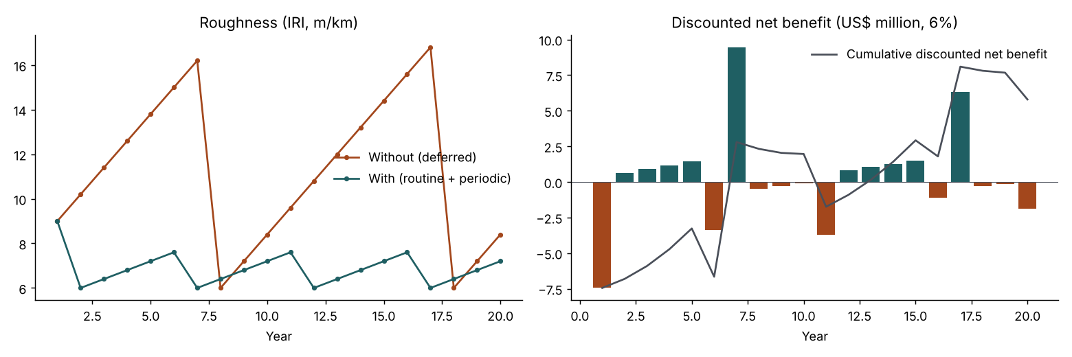
The trajectory of net benefits fluctuates considerably across the project lifecycle: regravelling years (Years 1, 6, 11, and 16) require heavy capital outlays and generate negative net annual balances. Conversely, Years 7 and 17—when deferred maintenance would have triggered costly full reconstructions—exhibit substantial positive peaks. Interestingly, in Years 8 and 18, immediately following counterfactual reconstructions, the unmaintained road is temporarily smoother than the maintained surface, resulting in slight, transient net negative user benefits in those two years.
Switching values analysis
| Parameter Tested (all others at baseline) | Baseline Value | Switching Value (NPV = 0) | Critical Variance |
|---|---|---|---|
| Initial traffic, Year 1 | 120 veh/day | 89.7 veh/day | −25% |
| VOC response slope | 0.013 | 0.0091 | −30% |
| Unit cost of regravelling | US$18,000/km | US$23,581/km | +31% |
| Capital cost overrun | 10% | 32.9% | +22.9 points |
| Annual traffic growth rate | 4.0% | 0.5% | −3.5 points |
| Avoided reconstruction cost | US$30,000/km | US$9,948/km | −67% |
| Deterioration rate without maintenance | 1.2 IRI/yr | ~0.65 IRI/yr | ~−46% |
| Value of travel time | US$1.0/person-hr | Zero | NPV remains US$1.33 million |
| All project benefits combined | — | — | −17% |
| All project costs combined | — | — | +21% |
| Critical discount rate | 6% | 14.7% (EIRR) | +8.7 points |
The relationship between asset deterioration rates and project NPV is non-monotonic due to the discrete timing of reconstruction triggers; the NPV profile crosses the break-even line multiple times between 0.60 and 0.70 IRI per year. The practical policy takeaway is robust: proactive maintenance is not economically warranted if the unmaintained gravel pavement deteriorates at a rate below approximately 0.7 IRI per year.
Sensitivity analysis and Monte Carlo simulation
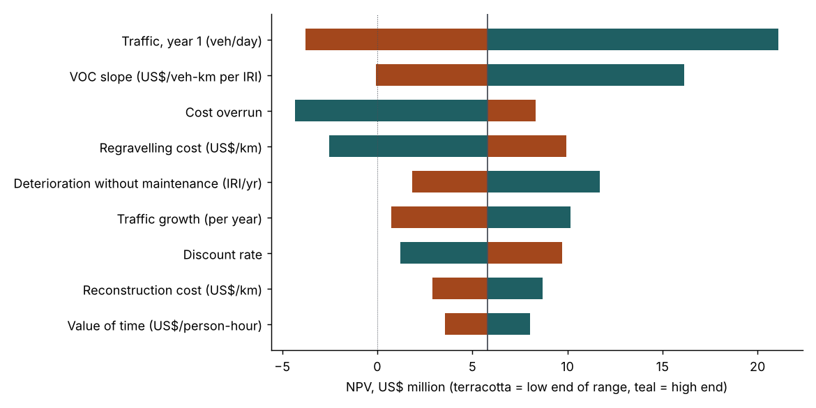
Initial traffic volume represents the dominant source of project variance: NPV spans from −US21.09 million at 200 veh/day. The sensitivity of VOC savings to roughness, civil works cost overruns, and regravelling unit rates form the next tier of influential parameters.
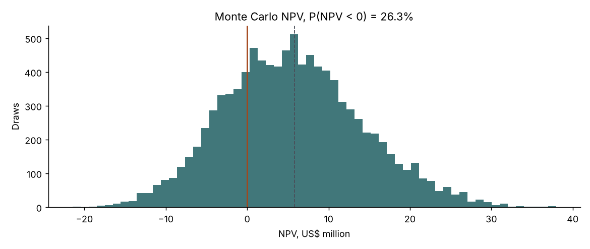
A probabilistic Monte Carlo simulation sampling eight independent triangular distributions across 10,000 iterations (seed: 20261103; discount rate held at 6%) yields a mean NPV of US5.34 million. The 5th to 95th percentile interval ranges from −US20.65 million, with . Spearman rank correlations confirm the structural ranking shown in the tornado diagram: traffic volume (0.64), VOC slope (0.41), regravelling unit cost (−0.34), and cost overruns (−0.34). Parameter independence is an analytical simplification; in operational contexts, traffic growth and asset wear are positively correlated, which would widen the distribution's tails.
Distributional and fiscal analysis
Distribution of economic gains. The overwhelming majority of project benefits accrue to direct road users: transport operators through reduced maintenance costs, passengers through shortened journey times, and local populations through newly generated mobility. The degree to which these cost reductions benefit agricultural producers and rural households depends on market pass-through into local transport fares and freight rates, which is governed by the competitiveness of the local trucking sector. Furthermore, because economic benefits scale with traffic density, ranking networks strictly by NPV prioritizes busier, better-connected links. Where public policy aims to improve access for marginalized or impoverished areas, this should be incorporated as an explicit spatial equity criterion—in line with the UK Green Book’s distributional appraisal guidelines (para. 2.28)—rather than hidden through ad hoc adjustments to the discount rate.
Fiscal commitments and budgetary risk. The road authority bears the entirety of program costs. In nominal financial terms (including baseline overruns), the programme demands an average annual outlay of US6,600/km): comprising US1.58 million, and US9.5 million to clear maintenance backlogs. By comparison, deferred maintenance requires only US12 million every ten years (averaging US$1.4 million annually).
Crucially, the programme shifts expenditure from episodic capital projects—frequently funded by external multilateral donors—to steady recurrent liabilities that must be secured through national road funds or domestic revenue allocations. Approving such a scheme without ring-fenced recurrent funding guarantees institutional drift back into deferred maintenance, forfeiting the economic benefits modeled here.
Methodological limitations
- Single composite fleet model: The framework employs a linear VOC relationship for an average vehicle rather than disaggregated HDM-4 models segmented by commercial vehicle class and local factor prices. Heavy commercial vehicle operating costs typically rise more steeply with roughness than passenger cars.
- Omission of broader social externalities: The analysis does not monetize the benefits of assured all-weather accessibility during rainy seasons, road safety improvements, non-motorized transport, or enhanced access to rural health and education centers.
- Traffic-invariant maintenance costs: Routine maintenance expenditure is modeled as fixed per kilometre rather than indexing against cumulative equivalent standard axles.
- Illustrative unit costs: The cost data represent scalable benchmarks rather than site-specific contractor price surveys.
- Stochastic independence assumptions: The Monte Carlo engine samples input distributions independently, omitting structural covariances between macroeconomic factors and operational costs.
Implementation pathway for operational programmes
In an operational deployment, analysts would substitute the synthetic network with link-level classified traffic counts and visual pavement distress surveys, run localized RED or HDM-4 engines, and prioritize links by NPV per kilometre—allocating funds first to corridors that comfortably exceed the switching-value traffic thresholds.
The switching-value schedule represents the most valuable decision-support tool for ministerial dialogue: it reduces the economic appraisal to a concise checklist of empirical realities to verify (verified traffic counts, contracted regravelling rates, and documented deterioration curves) prior to capital commitment. Following commissioning, annual roughness assessments (using calibrated smartphone bump integrators or response-type meters) alongside sample traffic audits should be conducted to verify that actual performance matches the modeled trajectory.